Legend has it that mere moments after inventing the bicycle in 1817, Karl von Drais tried riding it up a steep hill and, recognizing how miserable a task he’d embarked upon, exclaimed, “Well, this freakin’ sucks.”
It’s possible von Drais didn’t actually say that, but I certainly thought it recently when I tried taking a CitiBike uphill in my hometown of Park Slope, a neigborhood quite literally named after its characteristic gradient. I imagined how free and easy the opposite route would be – I could probably ride the descent down from Prospect Park without even pedaling.
Indeed, if you query the data that CitiBike makes available, you’ll find that riders making my same arduous journey up Third Street across several avenues did so in about three and a half minutes, while riders going in the other direction between those two stations took only about two and a half minutes on average. This data only provides ride duration and no actual time series of position or velocity, but we can still calculate effective “straight-line” speeds of 5.8 and 7.6 miles per hour, respectively, once we determine the stations are 0.33 miles apart.
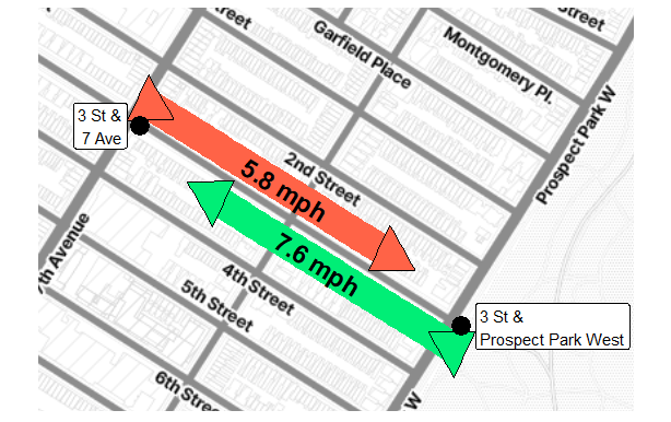
How well does this idea scale, though? If the hill between Prospect Park West and 7th Avenue leaves a signature in CitiBike data, is the difference in elevation between any two endpoints embedded in the net speed achieved by bikers riding between them? Nearly half of Brooklyn is covered in a dense lattice of over 700 CitiBike stations that accounted for millions of rides in 2024. Is the data that system generates enough to reverse-engineer a topographic map of the borough?
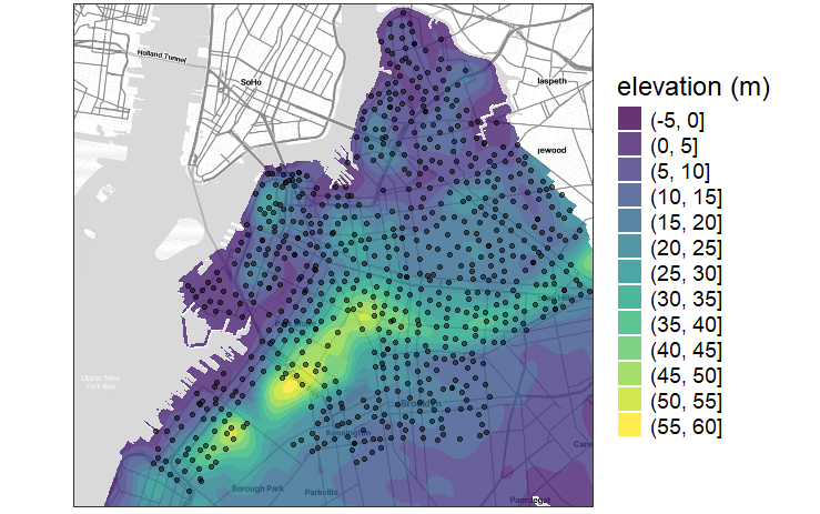
First, let’s examine an actual topographic map of Brooklyn overlaid with the locations of CitiBike stations. The aforementioned hill that peaks along the west side of Prospect Park is part of a larger ridge that starts in Sunset Park, extends northeast into Prospect Heights, and then turns east through Crown Heights. There are also more isolated patches of elevation in Carroll Gardens, Downtown Brooklyn, and Williamsburg. The map bottoms out along the waterfront and in the Gowanus region. Any elevation patterns in the southeast corner will not be recoverable in our experiment since there are no stations there.
We define a few rules to help us home in on true traveling speeds via bicycle:
As before, all speeds are expressed in “straight-line” terms, even though bikers obviously must use the roads available to them in lieu of crashing through residential homes or flying over them. The hope is that the effect of hills is strong enough to overcome our lack of precise tracking data or intuitive routing.
Rides must be on the old-school manual bikes. The new, increasingly popular e-bikes make it much easier to resist the pull of gravity, which risks muting the very pattern we’re looking for.
Rides must be taken by subscribers and not single-pass users. Repeat riders are more likely to be using the bike for practical reasons while the one-off renters might be tourists looking for a leisurely, scenic ride.
Distances between stations cannot be longer than a mile. This constraint helps us reduce the data size and also likely protects us from longer journeys which could feature more indirect routes.
Rides must achieve a straight-line speed of at least 3 MPH and at most 30 MPH. If you are going slower than that, you’re likely not trying to get from Point A to Point B with any haste (in fact many renters return their bike at or near the starting point after meandering around the local area). If you’re going faster than that, the data is likely corrupt or you’re a world-class cyclist ripping through crowded urban areas – please slow down, sir.
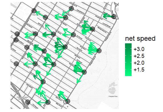
Once we’ve applied these filters, speeds in both directions between any pair of stations are easy to calculate. Below is a vector field of net speeds in Park Slope. The arrows point through the gridded streets instead of exclusively along them thanks to Rule # 1, which pretends that bikers ride “as the crow flies.” In any case, they generally point down from the park, which is a good early sign.
So how are we going to back into elevation coordinates for CitiBike stations from these speed comparisons? The key is to assume that there’s some sort of positive relationship between going downhill and going faster, and then iteratively increase that correlation by adjusting the elevation data until we can no longer make any meaningful improvements. In other words, we’ve observed speed differences in various directions and now need to mold a surface to better explain them.
In more technical terms, this is a high-dimensional optimization problem. Our unknown parameters are the 700 or so elevations of our CitiBike stations. The loss function is the goodness of fit (in our case, the average squared residual) for a linear model regressing net speed between stations on the difference in elevation implied by those input parameters.
Here is a composite visualization of the optimization’s first 200 iterations. From left to right, the elevations are updated, leading to an increasingly precise relationship between the elevation difference and net speed achieved between all pairs of stations, which drives down our assessment criteria and informs the algorithm how to further update the elevations.
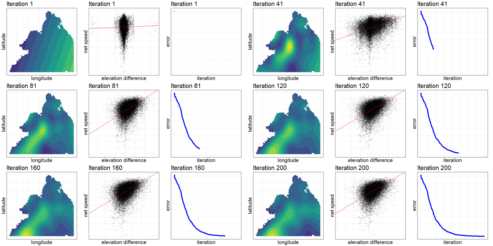
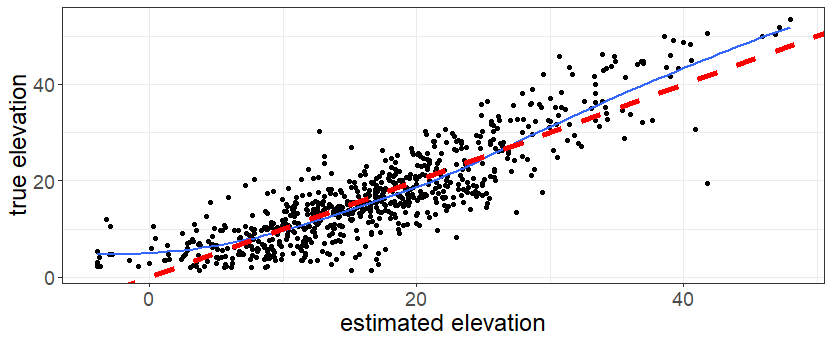
After a thousand iterations and many hours of torching my processor with parallel computing, the optimization is complete, or at least good enough. The results are surprisingly accurate. Once you put the optimized parameters on the same scale as the actual CitiBike elevations (which we can look up), 69% of our estimates are within five meters of the true figures, good for 87% correlation.
The big misses, such as the conspicuous one in the bottom right of the scatterplot, are intriguing in their own right. The algorithm thinks the station on Johnson St. and Brooklyn Bridge Boulevard sits atop a 42-meter peak based on the high speed achieved by bikers riding away from it. But in reality, the routes leading into that station are simply much more indirect thanks to one-way streets, confusing the model into thinking they are uphill. Errors like this would be reduced if we had access to actual traveling speeds of the bikes instead of just trip durations.
And finally, we can plug these implied station elevations into a 2D-smoother to build a contour map. We get something that’s not quite as peaked as the actual topographic map, which makes sense when relying on a coarser data set, but still pretty similar to the original. Here are the two side-by-side.
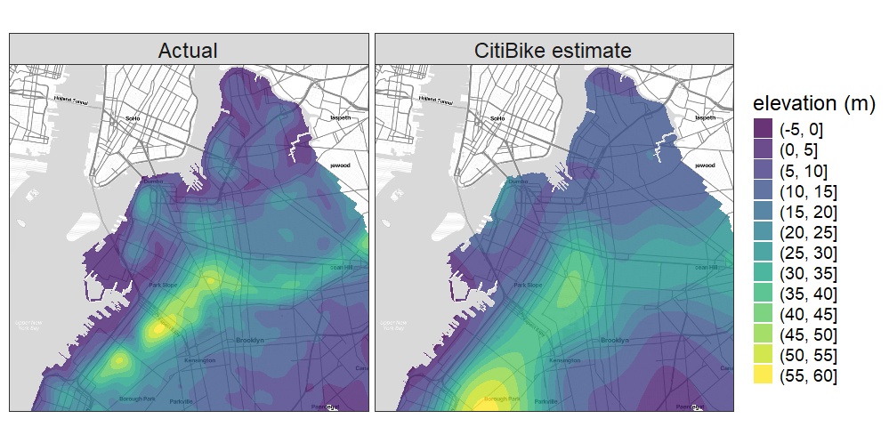
Functionally there’s no use for this map when real elevations are readily available. But I find the idea that we could recreate a topographic map with just CitiBike data at once simple and also fascinating. The concept of gravity is so fundamental that it’s actually hidden in a dataset that has no explicit definition of gradient or elevation– so that by sharing its ride data in an attempt to publish useful information about a public transportation resource, CitiBike was unknowingly handing over a contour map of the city.
And this of course is the beauty of data sciences in general: there are profound patterns expressed somewhere in our datasets. We just have to work hard – not unlike an uphill rider – to find them.
All code used to analyze the data and display the results can be found below. Thanks for reading!
Code
########## setup ##########

library(tidyverse)
library(data.table)
library(glue)
library(ggmap)
library(sf)
library(httr)
library(mgcv)
library(optimParallel)
library(gridExtra)
library(gganimate)
library(magick)

# ways to make dplyr stfu
options(dplyr.summarise.inform = FALSE)
inner_join <- function(...) dplyr::inner_join(relationship = "many-to-many", ...)

# necessary when downloading files from internet
temp_file_path <- tempfile(fileext = ".zip")
temp_dir <- tempdir()

# api keys
google_elevation_key <- "xXxXxXxXxXxX"
register_stadiamaps(key = "yYyYyYyYyYyY")

cl <- makeCluster(detectCores())     # set the number of processor cores
setDefaultCluster(cl = cl) # set 'cl' as default cluster

# update and save this list throughout script
# only use for stuff that takes a long time or might not be accessible later (url or APIs)
# imagine needing to run it in 5 minutes without the internet

important_stuff <- list()
if(file.exists("important_stuff.Rdata")) load("important_stuff.Rdata")
list2env(important_stuff, globalenv())

########## retrieve data from online ##########

# brooklyn coordinates
left <- -74.05
bottom <- 40.63
right <- -73.9
top <- 40.74

# zoomed brooklyn coordinates
leftz <- -73.99
bottomz <- 40.66
rightz <- -73.97
topz <- 40.675

if(!exists("maps")){

  map_bk <- get_map(c(left = left,
                      bottom = bottom,
                      right = right,
                      top = top),
                    source = "stadia",
                    maptype = "stamen_toner_lite")

  map_bk_zoom <- get_map(c(left = leftz,
                           bottom = bottomz,
                           right = rightz,
                           top = topz),
                         source = "stadia",
                         maptype = "stamen_toner_lite")

  maps <- list(map_bk = map_bk, map_bk_zoom = map_bk_zoom)


  important_stuff$maps <- maps
}


if(!exists("brooklyn")){

  # read in borough shape files from govt site

  boro_url <- "https://data.cityofnewyork.us/api/geospatial/tqmj-j8zm?method=export&format=Shapefile"
  download.file(boro_url, destfile = temp_file_path, mode = "wb")
  unzip(temp_file_path, exdir = temp_dir)

  boros <- read_sf(temp_dir)
  brooklyn <- boros %>% filter(boro_name == "Brooklyn")

  important_stuff$brooklyn <- brooklyn
}


if(!exists("trips_raw_classic")){

  # create urls, accounting for crappy naming convention
  months <- str_pad(1:11, width = 2, pad = "0")
  extra <- rep("", length(months))
  extra[1:4] <- ".csv"
  urls <- glue("https://s3.amazonaws.com/tripdata/2024{months}-citibike-tripdata{extra}.zip")

  # must unzip file of CSVs for every url
  trips_raw <- map(urls, ~{

    download.file(.x, destfile = temp_file_path, mode = "wb")
    unzip(temp_file_path, exdir = temp_dir)

    csvs <- list.files(temp_dir, recursive = TRUE, full.names = TRUE) %>% keep(~str_detect(.x, "csv"))
    d <- csvs %>% map(fread) %>% bind_rows()

    file.remove(csvs)
    gc()

    d

  }) %>%
    bind_rows()

  # only care about manual member rides, ditch rest for memory purposes
  trips_raw_classic <- trips_raw %>% filter(rideable_type == "classic_bike", member_casual == "member")
  rm(trips_raw)
  gc()

  important_stuff$trips_raw_classic <- trips_raw_classic
}

########## summarize trip data ##########

stations <- trips_raw_classic %>%
  group_by(station_id = start_station_id, station_name = start_station_name) %>%
  summarize(
    # slight variation in coordinates within station
    lng = mean(start_lng),
    lat = mean(start_lat)
  ) %>%
  ungroup()

# convert stations to sf object
stations_sf <- stations %>%
  select(lat, lng) %>%
  st_as_sf(coords = c("lng", "lat"),
           crs = st_crs(brooklyn)
  )

# find which stations intersect w brooklyn shape file
ix_idx <- unlist(st_intersects(brooklyn, stations_sf))
stations_bk <- stations %>% slice(ix_idx)
stations_bk_sf <- stations_sf %>% slice(ix_idx)

# calculate distances between each and convert to miles
dist_matrix <- geosphere::distm(stations_bk %>% select(lat, lng), fun = geosphere::distHaversine)

station_pairs <- stations_bk %>%
  set_names(paste0("start_", names(.))) %>%
  crossing(stations_bk %>% set_names(paste0("end_", names(.)))) %>%
  mutate(distance = 3.28084*as.numeric(matrix(dist_matrix, ncol = 1))/5280)

# filter for reasonably fast trips of less than a mile
trips <- trips_raw_classic %>%
  mutate(duration = as.numeric(ended_at - started_at)) %>%
  inner_join(station_pairs, by = c('start_station_name', 'start_station_id', 'end_station_name', 'end_station_id')) %>%
  mutate(speed = distance/(duration/3600)) %>%
  filter(speed >= 3, speed <= 30, distance < 1)

trips_by_station <- trips %>%
  group_by(start_station_id, start_station_name, end_station_id, end_station_name, distance) %>%
  summarize(n = n(), mean_speed = mean(speed)
  ) %>%
  ungroup()

# bilateral vereion of routes dataframe include both possible directions
trips_by_station_bd <- trips_by_station %>%
  inner_join(trips_by_station,
             by = c('start_station_id' = 'end_station_id',
                    'start_station_name' = 'end_station_name',
                    'end_station_id' = 'start_station_id',
                    'end_station_name' = 'start_station_name',
                    'distance'),
             suffix = c('_fromA', '_fromB')
  ) %>%
  rename(station_id_A = start_station_id,
         station_name_A = start_station_name,
         station_id_B = end_station_id,
         station_name_B = end_station_name) %>%
  # de-dupe rows by only taking the fast direction
  mutate(speed_diff = mean_speed_fromA - mean_speed_fromB,
         n_h = 2*n_fromA*n_fromB/(n_fromA + n_fromB)) %>%
  filter(speed_diff > 0)


# only need to consider stations that are actually used
stations_n <- trips_by_station_bd %>%
  group_by(station_id = station_id_A,
           station_name = station_name_A) %>%
  summarize(n_h_A = sum(n_h)) %>%
  full_join(
    trips_by_station_bd %>%
      group_by(station_id = station_id_B,
               station_name = station_name_B) %>%
      summarize(n_h_B = sum(n_h)),
    by = c("station_id", "station_name")) %>%
  transmute(station_id, station_name, n_h_station = coalesce(n_h_A, 0) + coalesce(n_h_B, 0))

stations_bk_used <- stations_bk %>%
  inner_join(stations_n, by = c("station_id", "station_name")) %>%
  mutate(station_idx = row_number())

# some better naming conventions
trips_by_station_bd <- trips_by_station_bd %>%
  inner_join(stations_bk_used, by = c('station_id_A' = 'station_id', 'station_name_A' = 'station_name')) %>%
  inner_join(stations_bk_used, by = c('station_id_B' = 'station_id', 'station_name_B' = 'station_name'),
             suffix = c("_A", "_B"))

########## add real elevation data ##########

if(!exists("brooklyn_grid")){

  # 10k point grid for finding actual elevations
  brooklyn_grid_box <- expand.grid(
    lng = seq(left, right, length.out = 100),
    lat = seq(bottom, top, length.out = 100)
  )

  # chunk into 200 since google API has limits per request
  brooklyn_grid <- brooklyn_grid_box %>%
    st_as_sf(coords = c("lng", "lat"),
             crs = st_crs(brooklyn)
    ) %>%
    st_intersects(brooklyn, .) %>%
    unlist() %>%
    slice(brooklyn_grid_box, .) %>%
    mutate(google_group = ceiling(row_number()/200))

  elev_reqs_bk <- brooklyn_grid %>%
    group_split(google_group) %>%
    map(~{

      print(.x$google_group[1])
      Sys.sleep(3)

      locations <- .x %>%
        mutate(location = paste0(lat, ",", lng)) %>%
        pull(location) %>%
        paste0(collapse = "|")

      elev_req <- GET(
        url = "https://maps.googleapis.com/maps/api/elevation/json",
        query = list(
          locations = locations,
          key = google_elevation_key
        )
      )

    })


  brooklyn_grid$elev <- elev_reqs_bk %>%
    map(~map_dbl(content(.x)$results, ~.x$elevation)) %>%
    unlist()

  important_stuff$brooklyn_grid <- brooklyn_grid
}

if(!exists("brooklyn_grid2")){

  # wildly overfit surface to create smoothed topographic map
  contour_real <- bam(elev ~ s(lng, lat, k = 500), data = brooklyn_grid, cluster = cl)

  # 1m point grid for smooth contours along brooklyn border/water
  brooklyn_grid2_box <- expand.grid(
    lng = seq(left, right, length.out = 1000),
    lat = seq(bottom, top, length.out = 1000)
  )

  brooklyn_grid2 <- brooklyn_grid2_box %>%
    st_as_sf(coords = c("lng", "lat"),
             crs = st_crs(brooklyn)
    ) %>%
    st_intersects(brooklyn, .) %>%
    unlist() %>%
    slice(brooklyn_grid2_box, .)

  brooklyn_grid2$pred_real <- predict(contour_real, newdata = brooklyn_grid2, cluster = cl)

  important_stuff$brooklyn_grid2 <- brooklyn_grid2

}

m1 <- ggmap(maps$map_bk) +
  geom_contour_filled(data = brooklyn_grid2,
                      aes(lng, lat, z = pred_real),
                      alpha = 0.8) +
  labs(fill = "elevation (m)") +
  theme_bw() +
  theme(axis.title = element_blank(),
        axis.text = element_blank(),
        axis.ticks = element_blank()) +
  theme(legend.title=element_text(size = 18),
        legend.text=element_text(size = 14))

m1_pts <- m1 +
  geom_point(data = stations_bk_used,
             aes(lng, lat),
             alpha = 0.5)

if(!exists("sbue")){

  # chunk into 200 since google API has limits per request
  sbue <- stations_bk_used %>% mutate(google_group = ceiling(row_number()/200))

  # getting actual elevations for the stations
  elev_reqs_citi <- sbue %>%
    group_split(google_group) %>%
    map(~{

      print(.x$google_group[1])
      Sys.sleep(3)

      locations <- .x %>%
        mutate(location = paste0(lat, ",", lng)) %>%
        pull(location) %>%
        paste0(collapse = "|")

      elev_req <- GET(
        url = "https://maps.googleapis.com/maps/api/elevation/json",
        query = list(
          locations = locations,
          key = google_elevation_key
        )
      )

    })


  sbue$elev <- elev_reqs_citi %>%
    map(~map_dbl(content(.x)$results, ~.x$elevation)) %>%
    unlist()

  important_stuff$sbue <- sbue
}

# contour based on actual elevations will give us sense of best possible map
contour_citi_actual <- gam(elev ~ s(lng, lat), data = sbue)

brooklyn_grid2 <- brooklyn_grid2 %>%
  mutate(pred_citi_actual = predict(contour_citi_actual, newdata = .))

m2 <- ggmap(maps$map_bk) +
  geom_contour_filled(data = brooklyn_grid2,
                      aes(lng, lat, z = pred_citi_actual),
                      alpha = 0.8)

########## optimization ##########

if(!exists("sbue2") | !exists("interm_vals")){

  sbue2 <- sbue %>% mutate(z = NA)

  clusterEvalQ(cl, library("tidyverse"))
  clusterExport(cl, c('sbue2', 'trips_by_station_bd'))

  # initiate with random values
  set.seed(1)
  x <- rnorm(nrow(sbue2) - 1)

  interm_vals_text <- capture.output(find_elev <- optimParallel(x, fn = function(x){

    # exponentiating to make elevation above ground (0)
    sbue2$z <- exp(c(x, 0))

    # look up height diff between pairs of stations
    tt <- trips_by_station_bd %>%
      mutate(zdiff = sbue2$z[station_idx_A] - sbue2$z[station_idx_B])

    s <- tryCatch({

      # fit a linear model regressing log of speed diff on height diff
      # constrain positive so that elevations aren't flipped
      mod <- nls(I(log(speed_diff)) ~ b0 + exp(b1)*zdiff,
                 data = tt,
                 weights = tt$n_h,
                 start = list(b0 = -1, b1 = 0))

      weighted.mean(residuals(mod)^2, mod$weights)

    },

    # if nls fails, return ridiculously high value to steer optimizer away
    error = function(cond) {
      return(1e10)
    })

    return(s)

  }, control = list(trace = 6, maxit = 1e1), method = "L-BFGS-B", lower = rep(-10, length(x)), upper = rep(7, length(x)))
  )

  # parse text for intermediate values
  interm_vals <- interm_vals_text %>%
    map(~str_extract(.x, "(?<=X =  ).+")) %>%
    keep(~!is.na(.x)) %>%
    map(~as.numeric(unlist(str_split(str_trim(.x), " ")))) %>%
    do.call(rbind, .)

  # final parameter
  sbue2$z <- exp(c(find_elev$par, 0))

  important_stuff$sbue2 <- sbue2
  important_stuff$interm_vals <- interm_vals
}

# put estimate on correct scale
sbue2 <- sbue2 %>%
  mutate(elev_est = predict(lm(elev ~ z, data = .)))

# compare estimates with actual elevations
c1 <- sbue2 %>%
  # summarize(cor(z, elev),
  #           mean(abs(elev_est - elev) < 5))
  ggplot(aes(elev_est, elev)) +
  geom_point() +
  geom_smooth(se = F) +
  geom_abline(col = "red", linetype = "dashed", linewidth = 2) +
  labs(x = "estimated elevation",
       y = "true elevation") +
  scale_x_continuous(breaks = c(0, 20, 40)) +
  scale_y_continuous(breaks = c(0, 20, 40)) +
  theme_bw() +
  theme(axis.title=element_text(size = 18),
        axis.text=element_text(size = 14))

# build final contour map using our estimates
contour_citi_est <- gam(elev_est ~ s(lng, lat), data = sbue2)

brooklyn_grid2 <- brooklyn_grid2 %>%
  mutate(pred_citi_est = predict(contour_citi_est, newdata = .))

# put predictions on same scale (preserve min, median, max of real pred)
brooklyn_grid2 <- brooklyn_grid2 %>%
  mutate(pred_citi_est2 = pred_citi_est - median(pred_citi_est)) %>%
  mutate(pred_citi_est2 = ifelse(pred_citi_est2 > 0, pred_citi_est2/max(pred_citi_est2), pred_citi_est2/abs(min(pred_citi_est2)))) %>%
  mutate(pred_citi_est2 = ifelse(pred_citi_est2 > 0, pred_citi_est2*(max(pred_real) - median(pred_real)), pred_citi_est2*(median(pred_real) - min(pred_real)))) %>%
  mutate(pred_citi_est2 = pred_citi_est2 + median(pred_real))

# comparison of real topographic map vs. our one from our estimates
b2l <- bind_rows(
  brooklyn_grid2 %>% transmute(lat, lng, type = "Actual", z = pred_real),
  brooklyn_grid2 %>% transmute(lat, lng, type = "CitiBike estimate", z = pred_citi_est2)
)

comp_wide <- ggmap(maps$map_bk) +
  geom_contour_filled(data = b2l,
                      aes(lng, lat, z = z),
                      alpha = 0.8) +
  facet_wrap(~type, nrow = 1) + labs(fill = "elevation (m)")  +
  theme_bw() +
  theme(axis.title = element_blank(),
        axis.text = element_blank(),
        axis.ticks = element_blank()) +
  theme(legend.title=element_text(size = 18),
        legend.text=element_text(size = 14),
        strip.text = element_text(size = 18))


comp_long <- ggmap(maps$map_bk) +
  geom_contour_filled(data = b2l,
                      aes(lng, lat, z = z),
                      alpha = 0.8) +
  facet_wrap(~type, nrow = 2) + labs(fill = "elevation (m)")  +
  theme_bw() +
  theme(axis.title = element_blank(),
        axis.text = element_blank(),
        axis.ticks = element_blank()) +
  theme(legend.title=element_text(size = 18),
        legend.text=element_text(size = 14),
        strip.text = element_text(size = 18))

########## animations ##########

gif_files <- c("anim_bg.gif", "anim_tt.gif", "anim_loss.gif")
# eventually progress is minimal
stop <- 200

if(sum(map_lgl(gif_files, file.exists)) < 3){

  tts <- coefs <- bgs <- loss <- list()

  for(i in 1:stop){

    # plug intermediate values through optim process

    x <- interm_vals[i, ]

    sbue_temp <- sbue2
    brooklyn_grid_temp <- brooklyn_grid

    sbue_temp$z <- exp(c(x, 0))

    tt <- trips_by_station_bd %>% mutate(zdiff = sbue_temp$z[station_idx_A] - sbue_temp$z[station_idx_B])


    mod <- nls(I(log(speed_diff)) ~ b0 + exp(b1)*zdiff,
               data = tt,
               weights = tt$n_h,
               start = list(b0 = -1, b1 = 0))

    contour_citi_est_temp <- gam(z ~ s(lng, lat), data = sbue_temp)

    brooklyn_grid_temp <- brooklyn_grid_temp %>%
      mutate(pred_citi_actual = predict(contour_citi_est_temp, newdata = .))

    # extract implied trips, contour map, coefficients, and loss
    bgs[[i]] <- brooklyn_grid_temp %>% mutate(iter = i)
    tts[[i]] <- tt %>% mutate(iter = i)
    coefs[[i]] <- c(coef(mod), "iter" = i)
    loss[[i]] <- c('resid' = weighted.mean(residuals(mod)^2, mod$weights), "iter" = i)

  }

  bgs_df <- bind_rows(bgs)
  tts_df <- bind_rows(tts)
  coefs_df <- bind_rows(coefs) %>% mutate(iter = as.integer(iter))

  # loss data needs progressive rows to show tail
  loss_df <- bind_rows(loss) %>% mutate(iter = as.integer(iter)) %>%
    arrange(desc(iter)) %>%
    slice(rep(1:nrow(.), 1:nrow(.))) %>%
    arrange(iter) %>%
    group_by(iter) %>%
    mutate(iter0 = stop - row_number() + 1) %>%
    {
      bind_rows(
        filter(., iter0 >= 2),
        filter(., iter0 == 2) %>% mutate(iter0 = 1)
      )
    }

  # create animations of contours, scatter plots, and loss function by iteration

  theme_bw2 <- theme_bw() +
    theme(axis.title = element_text(size = 25),
          plot.title = element_text(size = 30)) +
    theme(plot.margin = margin(5.5, 25.5, 5.5, 5.5, unit = "pt"))

  anim_bg <- {
    bgs_df %>%
      group_by(iter) %>%
      # need to normalize colors by frame
      mutate(pred_citi_actual = (pred_citi_actual - mean(pred_citi_actual))/sd(pred_citi_actual)) %>%
      ungroup() %>%
      ggplot(aes(lng, lat, z = pred_citi_actual)) +
      geom_contour_filled() +
      labs(title = 'Iteration {frame_time}',
           x = 'longitude',
           y = 'latitude') +
      theme_bw2 +
      transition_time(iter)
  } %>%
    animate(nframes = stop, height = 400, width = 400)

  anim_tt <- {
    tts_df %>%
      ggplot(aes(zdiff, log(speed_diff), size = n_h)) +
      geom_point(alpha = 0.1) +
      geom_abline(aes(intercept = b0, slope = exp(b1)),
                  data = coefs_df,
                  col = "red") +
      labs(title = 'Iteration {frame_time}',
           x = "elevation difference",
           y = "net speed") +
      theme_bw2 +
      transition_time(iter) +
      view_follow()
  } %>%
    animate(nframes = stop, height = 400, width = 400)

  anim_loss <- {
    loss_df %>%
      ggplot(aes(iter, resid)) +
      geom_line(col = "blue", linewidth = 2) +
      labs(title = 'Iteration {frame_time}',
           x = "iteration",
           y = "error") +
      theme_bw2 +
      theme(plot.margin = margin(5.5, 25.5, 5.5, 5.5, unit = "pt")) +
      transition_time(iter0)
  } %>%
    animate(nframes = stop, height = 400, width = 400)

  anim_save(gif_files[1], anim_bg)
  anim_save(gif_files[2], anim_tt)
  anim_save(gif_files[3], anim_loss)

}

combo_file <- "combo.gif"

if(!file.exists(combo_file)){
  # combine gifs into triptych
  anim_bg <- image_read(gif_files[1])
  anim_tt <- image_read(gif_files[2])
  anim_loss <- image_read(gif_files[3])

  combo_gif <- image_append(c(anim_bg[1], anim_tt[1], anim_loss[1]))

  for(i in 2:stop){
    combined <- image_append(c(anim_bg[i], anim_tt[i], anim_loss[i]))
    combo_gif <- c(combo_gif, combined)
  }

  anim_save(combo_file, combo_gif)
}

combo_gif <- image_read(combo_file)


########## extra graphs ##########

# two end points for park slope example
s1 <- "3865.05"
s2 <- "3905.15"

t <- trips_by_station %>%
  filter((start_station_id == s1 & end_station_id == s2) |
           (end_station_id == s1 & start_station_id == s2)
  ) %>%
  inner_join(trips_by_station,
             by = c('start_station_id' = 'end_station_id',
                    'end_station_id' = 'start_station_id',
                    'distance'),
             suffix = c('_fromA', '_fromB')
  ) %>%
  rename(station_id_A = start_station_id,
         station_id_B = end_station_id) %>%
  inner_join(stations_bk_used, by = c('station_id_A' = 'station_id')) %>%
  inner_join(stations_bk_used, by = c('station_id_B' = 'station_id'), suffix = c("_A", "_B"))

# a lot of this code is gross/hard-coded
# not easy to create custom visualizations without a package

# jittering points around so arrows don't overlap
tt <- t %>% mutate(lat_A = lat_A + (-1)^(row_number()) * 0.0003,
                   lat_B = lat_B + (-1)^(row_number()) * 0.0003) %>%
  # don't want full length
  mutate(lat_B2 = lat_A + 0.75*(lat_B - lat_A),
         lng_B2 = lng_A + 0.75*(lng_B - lng_A)) %>%
  # 5-10 degree adjustment since global coords screws it up a little
  mutate(angle = 180/pi*atan((lat_B - lat_A)/(lng_B - lng_A)) - 6)

l <- stations_bk_used %>%
  filter(station_id %in% c(s1, s2))

# putting text coordinates near middle and angling them in right direction
text_coords <- tt %>%
  transmute(lng_mid = lng_A + 0.6*(lng_B2 - lng_A),
            lat_mid = lat_A + 0.6*(lat_B2 - lat_A),
            angle,
            mean_speed_fromA
  ) %>%
  arrange(mean_speed_fromA)

# creating triangles since geom_segment is so ugly
width <- 0.0003

tris <- tt %>%
  select(station_id_A, lng_A, lat_A, lng_B2, lat_B2, angle) %>%
  # number of triangles
  crossing(tri = c(0, 3)) %>%
  # four points (repeat tip to close)
  crossing(data.frame(point = 0:3, tip = c(1, 0, 0, 1), anglediff = c(0, 90, -90, 0))) %>%
  mutate(anglep = angle + anglediff) %>%
  # this works just leave it alone
  mutate(lng_t = lng_A + (tri/3 + 0.15*tip-0.01)*(lng_B2 - lng_A) + (!tip)*width*cos((anglep * pi) / 180),
         lat_t = lat_A + (tri/3 + 0.15*tip-0.01)*(lat_B2 - lat_A) + (!tip)*width*sin((anglep * pi) / 180))


l$station_name <- str_replace_all(l$station_name, "& ", "&\n")

z1 <- ggmap(maps$map_bk_zoom) +
  geom_segment(data = tt, aes(x = lng_A, xend = lng_B2, y = lat_A, yend = lat_B2, col = as.factor(station_id_A)),
               linewidth = 10
  ) +
  geom_polygon(data = tris, aes(x = lng_t, y = lat_t, group = paste0(tri, station_id_A), fill = as.factor(station_id_A)), col = "black") +
  geom_point(aes(lng, lat), data = l, size = 6) +
  geom_label(aes(lng, lat, label = station_name),
             data = l %>% mutate(lng = lng + (-1)^(row_number()+1) * 0.0002),
             hjust = c(0, 1)) +
  scale_x_continuous(limits = c(-73.9795, -73.9715)) +
  scale_y_continuous(limits = c(40.6674, 40.6715)) +
  scale_color_manual(values = c("springgreen2", "tomato")) +
  scale_fill_manual(values = c("springgreen2", "tomato")) +
  theme(legend.position = "none") +
  theme(axis.title = element_blank(),
        axis.text = element_blank(),
        axis.ticks = element_blank())

for(i in 1:nrow(text_coords)){
  z1 <- z1 + annotate("text", x=text_coords$lng_mid[i], y=text_coords$lat_mid[i],
                      label = paste0(round(text_coords$mean_speed_fromA[i], 1), " mph"), color = "black",
                      angle = text_coords$angle[i], size = 6, fontface = "bold")
}

###############################################################

park_slope_stations <- c(4010.15, 3865.05, 3722.04, 3651.04, # ppw
                         3978.13, 3620.02, # 8th ave
                         3905.15, 3834.10, 3762.08, 3731.11, 3660.07, # 7th ave
                         4019.06, 3946.07, 3874.01, 3803.09, 3803.05, # 6th ave
                         3987.06, 3914.02, 3842.08, 3771.06, # 5th ave
                         4028.04, 3955.05, 3882.05) %>% # 4th ave
  as.character()

t <- trips_by_station_bd %>%
  filter(station_id_A %in% park_slope_stations, station_id_B %in% park_slope_stations,
         speed_diff > 1) %>%
  transmute(lat_A, lat_B, lng_A, lng_B, speed_diff,
            angle = atan((lat_B - lat_A)/(lng_B - lng_A))) %>%
  # new endpoints creating vectors of equal length
  mutate(lat_B2 = lat_A - 2/1000*sin(angle),
         lng_B2 = lng_A - 2/1000*cos(angle))

mps <- ggmap(maps$map_bk_zoom) +
  geom_segment(data = t, aes(x = lng_A, xend = lng_B2, y = lat_A, yend = lat_B2, col = speed_diff),
               linewidth = 1.25,
               arrow = arrow(length = unit(0.4, "cm"))
  )  +
  geom_point(data = stations_bk_used %>% filter(station_id %in% park_slope_stations), aes(lng, lat),
             size = 6, col = "black", fill = "black", pch = 21, alpha = 0.5) +
  scale_color_gradient(high = "springgreen4", low = "springgreen",
                       labels = scales::label_number(style_positive = c("plus")))+
  labs(col = "net speed") +
  theme(axis.title = element_blank(),
        axis.text = element_blank(),
        axis.ticks = element_blank()) +
  theme(legend.title=element_text(size = 18),
        legend.text=element_text(size = 14))

blog_graphs <- list(
  z1 = z1, m1_pts = m1_pts, mps = mps, c1 = c1, comp_wide = comp_wide, comp_long = comp_long
)

save(blog_graphs, file = "blog_graphs.Rdata")
save(important_stuff, file = "important_stuff.Rdata")